Cox regression, also referred to as proportional hazards regression, is one of the most widely used techniques in survival analysis. It is applied when the objective is to model the time until an event occurs while accounting for multiple predictor variables. In applied research, this event could be death, disease relapse, customer churn, equipment failure, or employee turnover. Researchers frequently rely on Cox regression when analyzing censored data, where the event has not occurred for all subjects during the observation period.
In applied statistics and health sciences, Cox regression is commonly performed using IBM SPSS Statistics because of its structured interface and robust survival analysis procedures. However, many researchers struggle with three core aspects: how to run Cox regression correctly in SPSS, how to handle time-dependent covariates, and how to interpret the output in a meaningful, real-world context.
This guide explains Cox regression in SPSS step by step, demonstrates real-life applications, and clarifies interpretation using practical examples. It also addresses advanced topics such as time-dependent Cox regression and common pitfalls encountered in academic and applied research.
What Is Cox Regression and When Should You Use It?
Cox regression is used when the dependent variable represents time to an event, and at least some observations are censored. Unlike linear or logistic regression, Cox regression focuses on the hazard function, which represents the instantaneous risk of the event occurring at a given time, assuming the individual has survived up to that time.
A defining feature of Cox regression is that it does not require specifying the baseline hazard function. This makes the model semi-parametric and particularly flexible for real-world data where the underlying time distribution is unknown or complex.
Typical use cases for Cox regression include medical studies evaluating patient survival after treatment, business analytics measuring time until customer churn, engineering reliability studies analyzing time to system failure, and social science research examining duration-based outcomes such as unemployment spells.
Cox regression is appropriate when the proportional hazards assumption is reasonably satisfied. This assumption implies that the effect of predictor variables on the hazard remains constant over time. Violations of this assumption require alternative modeling strategies, such as stratified models or time-dependent covariates.
How to Do Cox Regression in SPSS: Step-by-Step Procedure
Running Cox regression in SPSS involves careful data preparation and correct specification of variables. Errors at this stage often lead to invalid results or misinterpretation.
Step 1: Prepare the Dataset
Your dataset must contain a time variable that represents the duration until the event or censoring occurs. This could be measured in days, months, or years. You must also define a status variable indicating whether the event occurred or the observation was censored. The status variable is typically coded as 1 for event occurrence and 0 for censored cases.
Independent variables may include continuous predictors such as age or income, categorical predictors such as treatment group or gender, and binary indicators such as smoker versus non-smoker.
Step 2: Access the Cox Regression Dialog
In SPSS, navigate to Analyze, then Survival, and select Cox Regression. This opens the Cox regression dialog box where variables are assigned to their respective roles.
Step 3: Specify Time and Status Variables
Move the time variable into the Time field. Move the status variable into the Status field and define the event value correctly. Incorrect specification of the event value is one of the most common mistakes made by researchers.
Step 4: Add Covariates
Add all predictor variables into the Covariates box. For categorical variables, click the Categorical button and define reference categories appropriately. Failure to do so may result in misleading hazard ratio interpretations.
Step 5: Choose Method and Options
The default method, Enter, is suitable for most analyses. In the Options menu, request confidence intervals for hazard ratios and consider saving residuals for diagnostic checks.
Need Accurate Cox Regression Results in SPSS?
Don’t let censored data or time-dependent covariates stall your publication. Our experts handle model setup, assumption checks, and hazard ratio interpretation for defensible results.
✔ 1,000+ Projects Supported ✔ MSc & PhD Statistical Specialists ✔ Confidential & Supervisor-Ready Results ✔ Fast Turnaround ✔ Clear Reporting
Interpreting Cox Regression Output in SPSS
Correct interpretation of Cox regression results is essential for valid conclusions. The most critical component of the output is the Exp(B) column, which represents hazard ratios.
A hazard ratio greater than 1 indicates increased risk, while a value less than 1 indicates reduced risk. A hazard ratio equal to 1 suggests no effect. Confidence intervals must also be examined to assess statistical significance and estimate precision.
The Wald statistic and associated p-value indicate whether each predictor significantly affects survival time. However, statistical significance should always be interpreted alongside practical relevance.
For example, a hazard ratio of 1.02 may be statistically significant in large samples but have minimal real-world importance. Conversely, a hazard ratio of 2.5 represents a substantial effect that warrants attention even if the confidence interval is relatively wide.
Sample COX Regression results and interpretation
Interpretation
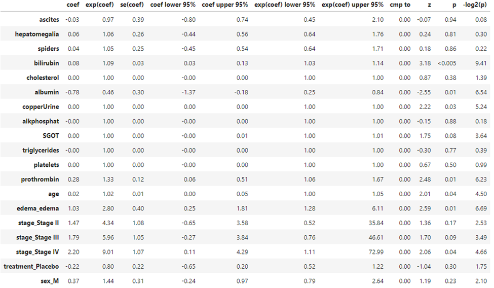
A Cox proportional hazards regression was conducted to determine the effect of several clinical and demographic variables on patient survival. The overall model identified bilirubin, albumin, copper urine, prothrombin time, age, edema, and Stage IV disease as significant predictors of the hazard rate (all $p < .05$).
Clinical Lab Findings
- Bilirubin: Higher bilirubin levels were significantly associated with an increased risk of the event ($HR = 1.09, 95\% CI [1.03, 1.14], p < .005$). For every one-unit increase in bilirubin, the hazard increased by 9%.
- Albumin: Albumin acted as a significant protective factor ($HR = 0.46, 95\% CI [0.25, 0.84], p = .01$). A one-unit increase in albumin was associated with a 54% reduction in the hazard.
- Prothrombin Time: Increased prothrombin time significantly increased the hazard ($HR = 1.33, 95\% CI [1.06, 1.67], p = .01$).
Demographics and Physical Findings
- Age: Age was a significant predictor ($HR = 1.02, 95\% CI [1.00, 1.05], p = .04$), indicating a 2% increase in risk for every year of age.
- Edema: The presence of edema was associated with a significantly higher hazard compared to those without edema ($HR = 2.80, 95\% CI [1.28, 6.11], p = .01$).
Disease Staging
The model utilized dummy coding for disease stages. Compared to the reference group (likely Stage I), only Stage IV reached statistical significance ($HR = 9.01, 95\% CI [1.11, 72.99], p = .04$). While Stage II and Stage III showed higher hazard ratios ($4.34$ and $5.96$ respectively), their confidence intervals crossed $1.0$, and their $p$-values ($p = .17$ and $p = .09$) did not meet the threshold for significance.
Findings Table
| Variable | B | SE | HR | 95% CI | p |
| Bilirubin | 0.08 | 0.03 | 1.09 | [1.03, 1.14] | < .005 |
| Albumin | -0.78 | 0.30 | 0.46 | [0.25, 0.84] | .01 |
| Prothrombin | 0.28 | 0.12 | 1.33 | [1.06, 1.67] | .01 |
| Age | 0.02 | 0.01 | 1.02 | [1.00, 1.05] | .04 |
| Edema | 1.03 | 0.40 | 2.80 | [1.28, 6.11] | .01 |
| Stage IV | 2.20 | 1.07 | 9.01 | [1.11, 72.99] | .04 |
Discussion Point
Notably, the Treatment (Placebo) group did not show a statistically significant difference from the treatment group ($p = .30$), suggesting that, after controlling for other clinical factors, the specific treatment administered in this dataset did not significantly alter the hazard of the event.
Time Dependent Cox Regression in SPSS
Time dependent Cox regression is required when the effect of a predictor changes over time or when a variable itself varies during the observation period. Examples include treatment dosage changes, employment status updates, or evolving health conditions.
SPSS does not provide a fully automated interface for time dependent Cox regression, but it can be implemented through data restructuring. This typically involves splitting each subject’s survival time into multiple intervals, with updated covariate values for each interval.
For example, in a workplace injury study, safety training may be introduced halfway through the observation period. By splitting the survival time into pre-training and post-training intervals, the analyst can model how training alters hazard rates over time.
Customer Churn Analysis Using Cox Regression
A subscription-based company tracks how long customers remain active before canceling their service. The time variable is measured in months from signup to churn or censoring. Predictors include subscription type, monthly usage, customer support interactions, and promotional discounts.
Cox regression reveals that high usage reduces churn risk, with a hazard ratio of 0.62, while frequent support complaints increase churn risk with a hazard ratio of 1.88. These findings guide retention strategies by identifying high-risk customer segments and actionable intervention points.
Assumptions and Diagnostic Checks
Cox regression relies on the proportional hazards assumption. Violations occur when hazard ratios change over time. Diagnostic checks such as log-minus-log plots or time interaction terms help assess this assumption.
Multicollinearity among predictors can distort hazard ratio estimates and should be evaluated using correlation matrices or variance inflation factors before modeling. Additionally, sample size adequacy is critical, as survival models with too few events produce unstable estimates.
Final Thoughts
Cox regression in SPSS is a powerful analytical technique for modeling survival and duration-based outcomes across disciplines. When applied correctly, it provides interpretable and actionable insights into risk factors influencing time-to-event processes. By understanding how to run Cox regression, interpret hazard ratios, and apply time dependent extensions, researchers can produce results that are both statistically rigorous and practically meaningful.