A normality test in SPSS plays a central role in statistical decision-making. Many inferential procedures in SPSS, including paired sample t-tests, ANOVA, regression and Pearson correlation, rely on the assumption that the underlying data follow a normal distribution. When researchers ignore this assumption, they risk inaccurate p-values, misleading confidence intervals, and incorrect conclusions. For students, analysts, and researchers, understanding how to test for normality in SPSS and how to interpret test of normality output correctly determines whether parametric methods remain valid or whether nonparametric alternatives should be selected.
This guide explains data normality testing in SPSS in a practical, applied manner. You will learn how to run normality tests in SPSS using Shapiro–Wilk, Kolmogorov–Smirnov, skewness, kurtosis, histograms, Q–Q plots and boxplots. You will also learn how to interpret normality test SPSS results correctly for ANOVA and regression contexts, including small and large samples. Every section uses direct instructions, clear interpretation rules, and SPSS syntax so you can replicate the analysis without confusion.
What Is a Normality Test?
A normality test evaluates whether a variable follows a normal (Gaussian) distribution. In a normal distribution, values cluster symmetrically around the mean, with predictable spread and shape. Many statistical models assume this structure because it ensures valid standard errors and test statistics.
SPSS provides both numerical and graphical tools to test normality. Numerical tests include the Shapiro–Wilk normality test SPSS and the Kolmogorov–Smirnov normality test SPSS. Descriptive indicators such as skewness and kurtosis quantify distribution shape. Visual tools such as histograms and Q–Q plots allow researchers to detect deviations that significance tests may exaggerate in large samples.
A proper normality assessment never relies on a single statistic. Analysts combine test statistics, descriptive measures, and visual inspection to reach defensible conclusions.
How to Test for Normality in SPSS (Step-by-Step)
Method 1: Test of Normality via Explore
This method provides Shapiro–Wilk, Kolmogorov–Smirnov, skewness, kurtosis, and plots in one procedure.
Steps
- Click Analyze → Descriptive Statistics → Explore.
- Move the dependent variable into the Dependent List.
- Click Plots.
- Check Normality plots with tests.
- Click Continue, then OK.
SPSS produces a Test of Normality table, descriptive statistics, histograms, and Q–Q plots.
SPSS Syntax
EXAMINE VARIABLES=your_variable
  /PLOT BOXPLOT HISTOGRAM NPPLOT
  /COMPARE GROUP
  /STATISTICS DESCRIPTIVES
  /CINTERVAL 95
  /MISSING LISTWISE.
Shapiro–Wilk Normality Test SPSS
The Shapiro–Wilk normality test offers the most reliable performance for small and moderate sample sizes. Researchers commonly apply it when sample size remains below 2000.
Interpretation Rule
- Sig. > 0.05 indicates no statistically significant deviation from normality.
- Sig. ≤ 0.05 indicates a statistically significant deviation from normality.
Shapiro–Wilk often flags non-normality in real-world data, so analysts must confirm results with skewness, kurtosis, and plots.
SPSS Syntax (Shapiro–Wilk)
The Explore procedure automatically produces Shapiro–Wilk results. SPSS does not provide a standalone command for Shapiro–Wilk.
Kolmogorov–Smirnov Normality Test SPSS
The Kolmogorov–Smirnov normality test compares the empirical distribution of the data with a theoretical normal distribution. Researchers frequently use it for large samples.
Interpretation Rule
- Sig. > 0.05 suggests approximate normality.
- Sig. ≤ 0.05 suggests non-normality.
Large samples cause Kolmogorov–Smirnov to detect trivial deviations, so interpretation must rely on effect size and plots.
SPSS Syntax (Kolmogorov–Smirnov)
NPAR TESTS
  /ONESAMPLE KS=your_variable
  /MISSING ANALYSIS.
Normality Test Skewness and Kurtosis
Skewness measures asymmetry, while kurtosis measures peakedness or tail weight. SPSS reports both statistics and their standard errors.
Guidelines for Normality
- Skewness between −1 and +1 supports approximate normality.
- Kurtosis between −1 and +1 supports approximate normality.
Researchers often accept values up to ±2 in applied research, especially with larger samples.
SPSS Syntax
DESCRIPTIVES VARIABLES=your_variable
  /STATISTICS=MEAN STDDEV SKEWNESS KURTOSIS.
Interpreting Normality Test Output Correctly
Interpreting normality test SPSS output requires context. A statistically significant result does not automatically invalidate parametric analysis.
Best Practice Interpretation
- Combine Shapiro–Wilk or Kolmogorov–Smirnov with skewness, kurtosis, and Q–Q plots.
- Prioritize visual diagnostics for large samples.
- Focus on residual normality for regression and ANOVA, not raw variables.
When tests contradict plots, analysts should justify decisions transparently in the methodology section.
Normality Test SPSS for ANOVA
ANOVA assumes normally distributed residuals, not normally distributed raw group scores. Analysts must test residuals after fitting the model.
Steps
- Run ANOVA.
- Save standardized residuals.
- Test residuals using Explore.
SPSS Syntax (Save Residuals)
UNIANOVA dependent BY factor
  /SAVE RESID.
Multivariate Normality Test SPSS
SPSS does not provide a direct multivariate normality test. Analysts typically assess univariate normality first, then inspect Mahalanobis distances for multivariate outliers.
SPSS Syntax (Mahalanobis Distance)
REGRESSION
  /DEPENDENT y
  /METHOD=ENTER x1 x2 x3
  /SAVE MAHAL.
Outliers beyond the chi-square threshold suggest violations of multivariate normality.
Common Mistakes When Testing Normality
- Relying only on p-values
- Testing normality for categorical variables
- Ignoring residual-based normality
- Applying strict cutoffs without context
Avoiding these errors improves statistical credibility.
What to Do If Data Fail the Normality Test
When data violate normality assumptions, researchers can:
- Apply transformations (log, square root)
- Use nonparametric tests
- Rely on robust methods with large samples
Each decision must align with the research question and study design.
Conclusion
A normality test requires more than clicking a menu option. Accurate interpretation depends on understanding test behavior, sample size effects, and model assumptions. By combining Shapiro–Wilk, Kolmogorov–Smirnov, skewness, kurtosis, and visual diagnostics, researchers can justify statistical choices confidently. Correct normality testing strengthens credibility, improves inference, and prevents avoidable analytical errors in SPSS-based research.
Want Confidence in Your SPSS Results?
From assumption checks to final interpretation, our SPSS specialists help students present clean, defensible analyses that supervisors accept.


